import numpy as np3 NumPy arrays
3.1 Introduction
The NumPy package (module) is used in almost all numerical computations using Python. It is a package that provides high-performance vector, matrix and higher-dimensional data structures for Python. High-performance here refers to the fact that Python can perform computations on such data structures very quickly if appropriate functions are used for this.
To use NumPy you need to import the numpy module. This is typically done under the alias np so that you don’t have to type numpy all the time when using a function from the module.
We emphasize at this point that there is often not a unique way or command to achieve a certain outcome. When doing the exercises corresponding to the theory given in this chapter, it is, however, recommended to find a solution using the presented functionality.
3.2 Creating arrays
In the NumPy package the data type used for vectors, matrices and higher-dimensional data sets is an array, that can be created in various ways:
- a Python list or tuple;
- with functions that are dedicated to generating NumPy arrays, such as
np.arange()andnp.linspace()(we will see those later); - reading data from files.
We only discuss the first two options here.
3.2.1 Lists
For example, to create new vector and matrix arrays from Python lists we can use the numpy.array() function. Since we imported NumPy under the alias np, we use np.array() for this.
To create a vector, the argument to the array function is a Python list.
v = np.array([1,2,3,4]) #Array creation from list [1,2,3,4]
print(v)
[1 2 3 4]To create a matrix, the argument to the array function is a nested Python list. Every element of the outer list is a list corresponding to a row of the matrix. For example, the matrix M = \left[ \begin{matrix}1 & 2 & 7\\ 3 & -4 & 4 \end{matrix} \right] is created as follows.
M = np.array([[1, 2, 7], [3, -4, 4]])
print(M)
[[ 1 2 7]
[ 3 -4 4]]You can access the shape (number of rows and columns) , size (number of elements) and number of dimensions (number of axes in matrix) of the array with the np.shape(), np.size() and np.ndim() functions, respectively. Note that the size is simply the product of the numbers in the shape tuple, and the number of dimensions is the size of the shape tuple.
# Shape of matrix M
shape_M = np.shape(M)
print(shape_M)
(2, 3)# Size of matrix M
size_M = np.size(M)
print(size_M) 6# Number of dimensions
ndim_M = np.ndim(M)
print(ndim_M) 23.2.2 Special functions
There are various useful arrays that can be automatically created using functions from the NumPy package. These arrays are typically hard to implement directly as a list.
np.arange(n): This function creates the array [0,1,2,\dots,n-1] whose elements range from 0 to n-1.
n = 10
x = np.arange(n)

print(x)
[0 1 2 3 4 5 6 7 8 9]If you want to explicitly define the data type (floats, integers, etc.) of the elements, you can add the dtype keyword argument (the same applies for all functions that are given below), but you do not have to know this.
n = 10
x = np.arange(n)

print(x)
[0 1 2 3 4 5 6 7 8 9]# Numbers as floats
y = np.arange(n,dtype='float')
print(y)[0. 1. 2. 3. 4. 5. 6. 7. 8. 9.]np.arange(a,b): This function creates the array [a,a+1,a+2,\dots,b-2,b-1].
a, b = 5,11
x = np.arange(a,b)

print(x)
[ 5 6 7 8 9 10]np.arange(a,b,step): This function creates the array [a,a+step,a+2\cdot step,\dots,b-2\cdot step,b-step]. That is, the array ranges from a to b (but not including b itself), in steps of size step.
a, b, step = 5, 11, 0.3
x = np.arange(a,b,step)

print(x)
[ 5. 5.3 5.6 5.9 6.2 6.5 6.8 7.1 7.4 7.7 8. 8.3 8.6 8.9
9.2 9.5 9.8 10.1 10.4 10.7]np.linspace(a,b,k): Create a discretization of the interval [a,b] containing k evenly spaced points, including a and b as the first and last element of the array.
a,b,k = 5,10,20
x = np.linspace(a,b,k)

print(x)
[ 5. 5.26315789 5.52631579 5.78947368 6.05263158 6.31578947
6.57894737 6.84210526 7.10526316 7.36842105 7.63157895 7.89473684
8.15789474 8.42105263 8.68421053 8.94736842 9.21052632 9.47368421
9.73684211 10. ]np.diag(x): This function creates a matrix whose diagonal contains the list/vector/array x.
x = np.array([1,2,3])
D = np.diag(x)

print(D)
[[1 0 0]
[0 2 0]
[0 0 3]]np.zeros(n): This function create a vector of length n with zeros.
n = 5
x = np.zeros(n)

print(x)
[0. 0. 0. 0. 0.]np.zeros((m,n)): This function create a matrix of size m \times n with zeros. Note that we have to input the size of the matrix as a tuple (m,n). This is because the first input argument of np.zeros() should specify the size of the array (could be three- or higher-dimensional as well).
m, n = 2, 5
M = np.zeros((m,n))

print(M)
[[0. 0. 0. 0. 0.]
[0. 0. 0. 0. 0.]]If you would use np.zeros(m,n) then Python only sees m as the first input argument, and it does not what to do with the second argument n.
np.ones(n) and np.ones((m,n)): These functions create a vector of length n with ones, and a matrix of size m \times n with ones, respectively.
m, n = 2, 5
x = np.ones(n)

print(x)
[1. 1. 1. 1. 1.]M = np.ones((m,n))
print(M)[[1. 1. 1. 1. 1.]
[1. 1. 1. 1. 1.]]3.3 Accessing
In this section we will describe how you can access, or index, the data in a NumPy array.
We can index elements in an array using square brackets and indices just as we do with lists. In NumPy indexing starts at 0, again, just like with a Python list.
v = np.array([12,4,1,9])

# Element in position 0
print(v[0])

# Element in position 2
print(v[2])

# Element in position -1 (last element)
print(v[-1]) # Same as v[3]

# Element in position -3 (counted backwards)
print(v[-3]) # Same as v[1]
12
1
9
43.3.1 Basic indexing
If you want to access the element at position (i,j) from a two-dimensional array, you can use the double bracket notation [i][j], but with arrays you can also use the more compact syntax [i,j].
M = np.array([[10,2,6,7], [-15,6,7,-8], [9,10,11,12],[3,10,6,1]])

# Element at position (1,1)
print('List syntax:',M[1][1])

# Element at position (1,1)
print('Array syntax', M[1,1])
List syntax: 6
Array syntax 6If you want to access row i you can use M[i] or M[i,:].
print(M[2]) # Gives last row

print(M[2,:]) # Gives last row
[ 9 10 11 12]
[ 9 10 11 12]If you want to access column j you can use M[:,j]. Both here and in the previous command, the colon : is used to indicate that we want all the elements in the respective dimension. So M[:,j] should be interpreted as: We want the elements from all rows in the j-th column.
3.3.2 Index slicing
Index slicing is the technical name for the index syntax that returns a slice, a consecutive part of an array.
v = np.array([12,4,1,9,11,14,17,98])

print(v)
[12 4 1 9 11 14 17 98]v[lower:upper]: Returns the elements in v at positions lower, lower+1,...,upper-1. Note that the element at position upper is not included.
# Returns v[1], v[2], v[3], v[4], v[5]
print(v[1:6])
[ 4 1 9 11 14]You can also omit the lower or upper value, in which case it is set to be position 0 or the last position -1, respectively.
# Returns v[3],...,v[8]
print(v[3:])

# Returns v[0],...,v[4]
print(v[:5])
[ 9 11 14 17 98]
[12 4 1 9 11]v[lower:upper:step]: Returns elements in v at position
lower,lower+step,lower+2*step,...(upper-1)-step, (upper-1).
It does the same as [lower:upper], but now in steps of size step.
v = np.array([12,4,1,9,11,14,17,98])

# Returns v[1], v[3], v[5]
print(v[1:6:2])
[ 4 9 14]You can omit any of the three parameters lower,upper and step
# lower, upper, step all take the default values
print(v[::])

# Index in step is 2 with lower and upper defaults
print(v[::2])

# Index in steps of size 2 starting at position 3
print(v[3::2])
[12 4 1 9 11 14 17 98]
[12 1 11 17]
[ 9 14 98]You can also use slicing with negative index values.
# The last three elements of v
print(v[-3:])
[14 17 98]Furthermore, the same principles apply to two-dimensional arrays, where you can specify the desired indices for both dimensions
M = np.array([[10,2,6,7], [-15,6,7,-8], [9,10,11,12],[3,10,6,1]])

print(M)
[[ 10 2 6 7]
[-15 6 7 -8]
[ 9 10 11 12]
[ 3 10 6 1]]M[a:b, c:d]: Returns the submatrix of M consisting of the rows a,a+1,...,b-1 and columns c,c+1,...,d. You can also combine this with a step argument, i.e., use [a:b:step1, c:d:step2].
# Returns elements in submatrix formed by rows 2,3 (excluding 4)
# and columns 1,2 (excluding 3)
print(M[2:4,1:3])
[[10 11]
[10 6]]If you want to obtain a submatrix whose rows and/or columns do not form a consecutive range, or if you want to specify the indices manually, you can use the ix_() function from NumPy. Its arguments should be a list of row indices, and a list of column indices specifying the indices of the desired submatrix.
i = [0,2,3]
j = [0,3]

# Returns submatrix formed by rows 0,2,3 and columns 0,3
print(M[np.ix_(i,j)])
[[10 7]
[ 9 12]
[ 3 1]]3.3.3 Fancy indexing
Fancy indexing is the name for when an array or list is used instead of indices, to access part of an array. For example, if you want to access elements in the locations (0,3), (1,2) and (1,3), you can define a list of row indices [0,1,1] and columns indices [3,2,3] and access the matrix with these lists.
i = [0,1,1]
j = [3,2,3]

# Returns M[0,3] = 7, M[1,2] = 7, M[1,3] = -8
print(M[i,j])
[ 7 7 -8]Another way of fance indexing is by using a Boolean list, that indicates for every element whether it should be index (True) or not (False). Such a list is sometimes called a mask.
v = np.array([1,6,2,3,9,3,6])

# Tell for every element whether is should be index
mask = [False, True, True, True, False, True, False]

print(v[mask])
[6 2 3 3]Typically, the mask is generated from a Boolean statement. For example, suppose we want to select all elements strictly smaller than 3 and greater or equal than 7 from the array v.
The following statements achieve this. Recall that you can use & if you want the first AND the second statement to be satisfied, and | if either the first OR the second has to be satisfied (or both).
mask_37 = (v < 3) | (v >= 7)

# Boolean vector indiciating for ever element in v
# whether the conditions v < 3 and v >= 7 are satisfied
print(mask_37)
[ True False True False True False False]We can now access the elements satisfying these conditions by indexing v with this mask
print(v[mask_37])[1 2 9]3.4 Modifying
3.4.1 Elements, rows or columns
Using similar ways of indexing as in the previous section, we can also modify the elements of an array
M = np.array([[1,1,1,1], [2,2,2,2], [3,3,3,3],[4,4,4,4]])

print(M)
[[1 1 1 1]
[2 2 2 2]
[3 3 3 3]
[4 4 4 4]]# Modify individual element
M[0,1] = -1
print(M)[[ 1 -1 1 1]
[ 2 2 2 2]
[ 3 3 3 3]
[ 4 4 4 4]]# Modify (part of a) row
M[1,[1,2,3]] = [-2,-2,-2]
print(M)[[ 1 -1 1 1]
[ 2 -2 -2 -2]
[ 3 3 3 3]
[ 4 4 4 4]]# Modify third column to ones
M[:,3] = np.ones(4)
print(M)[[ 1 -1 1 1]
[ 2 -2 -2 1]
[ 3 3 3 1]
[ 4 4 4 1]]3.4.2 Broadcasting
There does not necessarily have to be a match between the part of the matrix that we index, and the dimensions of the data that we want to overwrite that part with.
M = np.array([[1,1,1,1], [2,2,2,2], [3,3,3,3],[4,4,4,4]])

print(M)
[[1 1 1 1]
[2 2 2 2]
[3 3 3 3]
[4 4 4 4]]For example, in order to replace the third column of M by ones, we can also do the command below, instead of using np.ones(4).
# Modify third column to ones
M[:,3] = 1

print(M)
[[1 1 1 1]
[2 2 2 1]
[3 3 3 1]
[4 4 4 1]]Although there is a mismatch between the indexed part on the left (a column) and the data on the right (a single number), Python broadcasts the data to an appopriate format by copying it to the correct size. That is, it copies the 1 to an array [1,1,1,1] of ones, which it then places in the third column.
This works similar in higher dimensions. Suppose we want to overwrite the second and third row with [1,6,2,3]. Then the indexed part is a 2 \times 4 array, but the data a 1 \times 4 array.
# Modify second and third row
M[2:4,:] = [1,6,2,3]

print(M)
[[1 1 1 1]
[2 2 2 1]
[1 6 2 3]
[1 6 2 3]]Python here first copies the data to [[1,6,2,3],[1,6,2,3]] and then modifies M with this array.
3.4.3 Transpose
Another useful function, in the context of linear algebra, is to take the transpose of a two-dimensional array M, which modifies the entries along the diagonal.
M = np.array([[1,2,3],[3,4,-1]])

print(M)
[[ 1 2 3]
[ 3 4 -1]]transpose_M = M.T #np.transpose(M) also works
print(transpose_M) [[ 1 3]
[ 2 4]
[ 3 -1]]3.5 Repeating and stacking
We can also use existing matrices and build new ones from it by stacking them either horizontally or vertically.
np.tile(M,(k,r)): This function takes an array M and copies it k times vertically and r times horizontally, resulting in a tiling of the original array M.
M = np.array([[1,2],[3,4]])

M_tile = np.tile(M,(2,3))
print(M_tile)
[[1 2 1 2 1 2]
[3 4 3 4 3 4]
[1 2 1 2 1 2]
[3 4 3 4 3 4]]If you do not input a tuples with two arguments, but only a number, then tile() does the tiling only horizontally.
M = np.array([[1,2],[3,4]])

M_tile = np.tile(M,4)
print(M_tile)
[[1 2 1 2 1 2 1 2]
[3 4 3 4 3 4 3 4]]np.repeat(M,k): This function takes every element of M, repeats it k times, and puts all these numbers in a one-dimensional array.
M = np.array([[1,2],[3,4]])

M_repeat = np.repeat(M,3)
print(M_repeat)
[1 1 1 2 2 2 3 3 3 4 4 4]vstack((a,b)): This stacks two arrays a and b vertically, provided they have the correct dimensions to do this. Note that a and b should be inputted as a tuple (a,b).
a = np.array([7,8])
M = np.array([[1,2],[3,4]])

M_a = np.vstack((M,a))
print(M_a)
[[1 2]
[3 4]
[7 8]]The reason that you have to use a tuple is similar as for np.zeros((m,n)). The first input argument of np.vstack() has to specify the input of what you want to stack. You can also stack more than two arrays if you give more than two inputs in the tuple.
a = np.array([7,8])
M = np.array([[1,2],[3,4]])
N = np.array([[11,12],[13,14]])

M_a_N = np.vstack((M,a,N))
print(M_a_N)
[[ 1 2]
[ 3 4]
[ 7 8]
[11 12]
[13 14]]np.hstack((a,b)): This stacks two arrays a and b horizontally, provided they have the correct dimensions to do this.
Note that in the example below we define a as a 1 \times 2 array, i.e., a column array, to make sure we can stack it right of M. If we would have kept a = np.array([7,8]) then Python will give an error, because it cannot stack a row vector next to a two-dimensional array.
a = np.array([[7],[8]])
M = np.array([[1,2],[3,4]])

M_a = np.hstack((M,a))
print(M_a)
[[1 2 7]
[3 4 8]]3.6 Reshaping
It is possible to adjust the shape of an array, while keeping the data of the array the same. For example, consider the array x = [1,2,3,\dots,12].
x = np.arange(1,13)

print(x)
[ 1 2 3 4 5 6 7 8 9 10 11 12]We can reshape it into the 3 \times 4 matrix
M = \left[ \begin{matrix} 1 & 2 & 3 & 4\\ 5 & 6 &7 & 8 \\ 11 & 10 & 11 & 12 \end{matrix}\right]
by using the reshape(a,b) method. It reshapes x to an a \times b array provided that a \cdot b equals the size (i.e., number of elements) of x.
# Reshape x to a 3-by-4 matrix
M = x.reshape(3,4)

print(M)
[[ 1 2 3 4]
[ 5 6 7 8]
[ 9 10 11 12]]We can also reshape two-dimensional arrays, for example, we can reshape M again to a 2 \times 6 matrix.
# Reshape M to a 2-by-6 matrix
N = M.reshape(2,6)

print(N)
[[ 1 2 3 4 5 6]
[ 7 8 9 10 11 12]]You should observe that Python does the reshaping in a very specific way: When we transform x to M above, Python fills the matrix M in a row-by-row fashion (instead of column-by-column). This is because of what is called the largest (axis) index changest fastest principle.
To understand this idea, recall that we can access the element at position (i,j) of a matrix M with M[i,j]. Here i is the row-index at position 0 of the index list [i,j], and j is the column index at position 1 of the index list [i,j]. We said that the row indices form the 0-axis of the matrix, and the column indices the 1-axis.
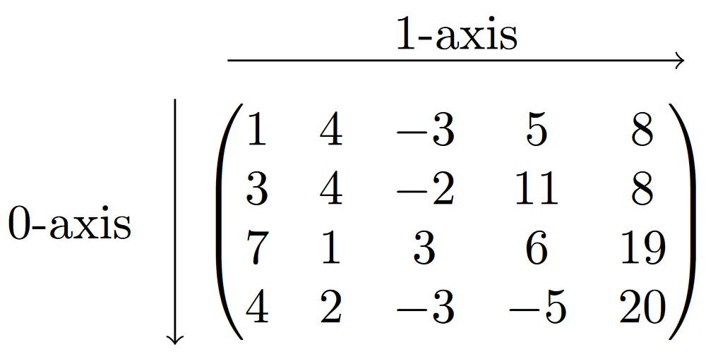
Largest (axis) index changing fastest means that an m \times n matrix gets filled first along the 1-axis, i.e., it fills the positions (0,0), (0,1), ..., (0,n) while keeping the row index 0 fixed. It then moves up one row index, i.e., one position along the 0-axis and fills the elements (1,0),(1,1),..., (1,n), i.e., the elements along the 1-axis. It continues in this fashion until the complete matrix is full.
Another convenient method for reshaping is flatten(), which turns a matrix of any size into a one-dimensional array.
# Define 2-by-3 matrix
M = np.array([[9,1,3],[2,4,3]])

# Turn into one-dimensional array
x = M.flatten()
print(x)
[9 1 3 2 4 3]If you want to turn a one-dimensional array x = [x_0,\dots,x_{n-1}] into a column array of shape (n,1), you can do this as follows.
x = np.array([1,2,4,3,8])
n = np.size(x)

x = x.reshape(n,1)
print(x)
[[1]
[2]
[4]
[3]
[8]]A more direct way of doing this, is by using x[:,None].
x = np.array([1,2,4,3,8])
x = x[:,None] # Turns x into column array of shape (n,1)

print(x)
[[1]
[2]
[4]
[3]
[8]]3.7 Copy vs. view
In the last sections we have seen various ways of using arrays to create other arrays. One point of caution here is whether or not the new array is a view or a copy of the original array.
3.7.1 View
A view y of an array x is another array that simply displays the elements of the array x in a different array, but the elements will always be the same. This means that if we would change an element in the array x, the same element will change in y and vice versa.
x = np.array([[4,2,6],[7,11,0]])
y = x # This create a view of x

print('y = \n', y)
y =
[[ 4 2 6]
[ 7 11 0]]We next change an element in x. Note that the same element changes in y.
# Change element in x
x[0,2] = -30

# y now also changes in that position
print('y = \n',y)
y =
[[ 4 2 -30]
[ 7 11 0]]The same happens the other way around: If we change an element in y, then the corresponding element in x also changes.
# Change element in y
y[1,1] = 100

# x now also changes in that position
print('x = \n', x)
x =
[[ 4 2 -30]
[ 7 100 0]]Note that the same behaviour occurs in we apply the reshape() method.
# Define x = [1,2,...,12]
x = np.arange(1,13)

# Reshape x to a 3-by-4 matrix
M = x.reshape(3,4) # Creates view of x

print(M)
[[ 1 2 3 4]
[ 5 6 7 8]
[ 9 10 11 12]]If we now change an element in M, then the corresponding element changes in x. This mean that M is a view of the original array x.
# Change element in M
M[1,3] = 50

# x now also changes in that position
print(x)
[ 1 2 3 4 5 6 7 50 9 10 11 12]3.7.2 Copy
A copy of an array x is an array z that is completely new and independent of x, meaning that if we change an element in x, then the corresponding element in z does not change, and vice versa. To obtain a copy of x, we can simply apply the copy() method to it.
# Define x = [1,2,...,12]
x = np.arange(1,13)

z = x.copy() # Create copy of x
z[0] = -10 # Change element of z

print('z = \n', z)
print('x = \n', x) # x has not changed
z =
[-10 2 3 4 5 6 7 8 9 10 11 12]
x =
[ 1 2 3 4 5 6 7 8 9 10 11 12]Note that in the above example, x remains unchanged when we modify the element of z at position 0.
Similarly, to turn a reshaped array into a copy, we can apply the copy() method to it.
# Define x = [1,2,...,12]
x = np.arange(1,13)

# Reshape x to a 3-by-4 matrix
M = x.reshape(3,4).copy() # Create copy
M[0,0] = -10 # Change element of x

print('M = \n', M)
print('x = \n', x) # x has not changed
M =
[[-10 2 3 4]
[ 5 6 7 8]
[ 9 10 11 12]]
x =
[ 1 2 3 4 5 6 7 8 9 10 11 12]The flatten() method actually directly creates a copy of the original array.
# Define 2-by-3 matrix
M = np.array([[9,1,3],[2,4,3]])

# Turn into one-dimensional array
x = M.flatten() # Creates copy of M
x[0] = 100 # Change element in x

print('x = \n', x)
print('M = \n', M) # M has not changed
x =
[100 1 3 2 4 3]
M =
[[9 1 3]
[2 4 3]]It is important to know whether a Python function or command creates a copy or a view of the original array. You can typically look this up in the documentation of Python. Otherwise, experiment with the function or command to be sure how it behaves.