from gurobipy import Model, GRB4 Linear optimization
In this chapter we will show how to implement linear optimization problems using Python. The goal is to model optimization problems in Python and then solve them using Gurobi, which is a software package dedicated to solving optimization problems. Note that it is important that you installed Gurobi correctly as explained in Chapter 2.
4.1 Basics
All the relevant functionality needed to use Gurobi via Python is contained in the gurobipy package. For our purposes, we only need two modules from this package:
- The
Modelmodule that we will use to build optimization problems - The
GRBmodule that contains various “constants” that we use to include words such as maximize and minimize.
In Python you can include the modules by adding the following line at the top of a script.
Example: Duplo problem
To illustrate how to implement optimization problems in Python, we consider the Duplo problem from the lectures: \begin{array}{llll} \text{maximize}& 15x_1 + 20x_2 && \text{(profit)} \\ \text{subject to} &x_1 + 2x_2 \leq 6 &&\text{(big bricks)} \\ &2x_1 + 2x_2 \leq 8 &&\text{(small bricks)} \\ &x_1, x_2 \geq 0 \end{array} with decision variables
- x_1: Number of chairs
- x_2: Number of tables
Let us implement the Duplo problem in Gurobi.
4.1.1 Model() object
To start, we will create a variable (or object) duplo that will contain all the information of the problem, such as the decision variables, objective function and constraints.
In programming terms, we create an object from the Model() class. We can give the instance a name by adding the name keyword argument, with value 'Duplo problem' in our case. We add this name with quotations so that Python knows this is plain text.
# Initialize Gurobi model.
duplo = Model(name='Duplo problem')
Set parameter Username
Set parameter LicenseID to value 2715549
Academic license - for non-commercial use only - expires 2026-09-29You can think of the Model class object duplo as a large box that we are going to fill with decision variables, an objective function, and constraints. We will also reserve a small space in this box to store information about the optimal solution to the linear optimization problem, once we have optimized the problem.
The concept of having “objects” is in fact what the programming language Python is centered around. This is known as object-oriented programming.
4.1.2 Decision variables
To add decision variables, an objective function, and constraints, to our Model object we use so-called methods which are Python functions.
To create a decision variable, we can use the addVar() method. As input argument, we include a name for the decision variables.
# Declare the two decision variables.
x1 = duplo.addVar(name='chairs')
x2 = duplo.addVar(name='tables')
If your Model object is not called
duplo, but for exampleproduction_planning, then you should useproduction_planning.addVar(name='chairs')instead. The same applies for all later methods that are introduced. Never call a modelModel(with capital M) because this spelling is reserved for theModel()class in Gurobi.
4.1.3 Objective function
Now that we have our decision variables, we can use them to define the objective function and the constraints.
We use the setObjective() method to do so by refering to the variables created above. The sense keyword argument must be used to specify whether we want to maximize or minimize the objective function. For this, we use GRB.MAXIMIZE or GRB.MINIMIZE, respectively.
# Specify the objective function.
duplo.setObjective(15*x1 + 20*x2, sense=GRB.MAXIMIZE)
4.1.4 Constraints
The next step is to declare the constraints using the addConstr() method. Also here, we can specify the constraints refering to the variables x1 and x2. We give the constraints a name as well.
# Add the resource constraints on bricks.
duplo.addConstr(x1 + 2*x2 <= 6, name='big-bricks')
duplo.addConstr(2*x1 + 2*x2 <= 8, name='small-bricks')
<gurobi.Constr *Awaiting Model Update*>We can also add the nonnegativity constraints x_1 \geq 0 and x_2 \geq 0 in this way, but this is actually not needed! By default, Python adds in the background the constraints that the decision variables should be nonnegative when creating them (see also Section 4.1.6).
4.1.5 Optimal solution
Now the model is completely specified, we are ready to compute the optimal solution. We can do this using the optimize() method applied to our model duplo.
# Optimize the model
duplo.optimize()
Gurobi Optimizer version 12.0.1 build v12.0.1rc0 (win64 - Windows 10.0 (19045.2))
CPU model: 12th Gen Intel(R) Core(TM) i7-1265U, instruction set [SSE2|AVX|AVX2]
Thread count: 10 physical cores, 12 logical processors, using up to 12 threads
Optimize a model with 2 rows, 2 columns and 4 nonzeros
Model fingerprint: 0xadc88607
Coefficient statistics:
Matrix range [1e+00, 2e+00]
Objective range [2e+01, 2e+01]
Bounds range [0e+00, 0e+00]
RHS range [6e+00, 8e+00]
Presolve time: 0.01s
Presolved: 2 rows, 2 columns, 4 nonzeros
Iteration Objective Primal Inf. Dual Inf. Time
0 3.5000000e+31 3.500000e+30 3.500000e+01 0s
2 7.0000000e+01 0.000000e+00 0.000000e+00 0s
Solved in 2 iterations and 0.01 seconds (0.00 work units)
Optimal objective 7.000000000e+01We can see some output from Gurobi, and the last line tells us that Gurobi found an optimal solution with objective value 70.
To summarize all the step above, we have given the complete code below (but not executed this time).
from gurobipy import Model, GRB

# Initialize Gurobi model.
duplo = Model(name='Duplo problem')

# Declare the two decision variables.
x1 = duplo.addVar(name='chairs')
x2 = duplo.addVar(name='tables')

# Specify the objective function.
duplo.setObjective(15*x1 + 20*x2, sense=GRB.MAXIMIZE)

# Add the resource constraints on bricks.
duplo.addConstr(x1 + 2*x2 <= 6, name='big-bricks')
duplo.addConstr(2*x1 + 2*x2 <= 8, name='small-bricks')

# Optimize the duplo
duplo.optimize()
Recalling our linear optimization problem object as being a “box” filled with decision variables, an objective function and constraints, the box now also contains a small space where the optimal solution is stored.
Let us have a look at how to access information about the optimal solution. The objective function value of the optimal solution, that was also displayed in the output when optimization the model with duplo.optimize() is stored in the ObjVal attribute. An attribute is a piece of information about an object in Python.
# Print text 'Objective value:' and the duplo.ObjVal attribute value
print('Objective value:', duplo.ObjVal)
Objective value: 70.0The optimal values of a decision variables can be obtained by accessing the X attribute of a variable.
print('x1 = ', x1.X)
print('x2 = ', x2.X)
x1 = 2.0
x2 = 2.0If the model has many variables, printing variables in this way is a cumbersome approach. It is then easier to iterate over all variables of the model using the getVars() method. This method creates a list of all the decision variables of the model.
print(duplo.getVars())[<gurobi.Var chairs (value 2.0)>, <gurobi.Var tables (value 2.0)>]As you can see above, we already see the optimal values of the decision variables, but also a lot of unnecessary information.
Let us print these values in a nicer format by iterating over the list duplo.getVars() using a for-loop with index variable var; you can choose another name here if you want. We print for every variable var its name, stored in the attribute VarName, and its value, stored in the attribute X. In between, we print the = symbol in plain text (hence, the quotations).
Recall that if you want to print multiple date types (such as a variables and text) in a print() statement, you should separate them with commas.
for var in duplo.getVars():
    print(var.VarName, "=", var.X)
chairs = 2.0
tables = 2.04.1.6 Help functionality
To see all these properties of method, e.g., addVar, you can check out the addVar documentation by typing help(Model.addVar) in Python. Looking up the documentation in this way can be done for every method.
help(Model.addVar)Help on cython_function_or_method in module gurobipy._model:
addVar(self, lb=0.0, ub=1e+100, obj=0.0, vtype='C', name='', column=None)
ROUTINE:
addVar(lb, ub, obj, vtype, name, column)
PURPOSE:
Add a variable to the model.
ARGUMENTS:
lb (float): Lower bound (default is zero)
ub (float): Upper bound (default is infinite)
obj (float): Objective coefficient (default is zero)
vtype (string): Variable type (default is GRB.CONTINUOUS)
name (string): Variable name (default is no name)
column (Column): Initial coefficients for column (default is None)
RETURN VALUE:
The created Var object.
EXAMPLE:
v = model.addVar(ub=2.0, name="NewVar")
For example, from this it can be seen that when creating a variable, you can specify more properties. You can use the keyword arguments lb and ub to define a lower and upper bound, respectively, for a decision variable.
If we would want to create a variable, with name Test variable, having lower bound 3 and upper bound 7, i.e., these bounds model the constraints x_1 \geq 3 and x_1 \leq 7, we can do this with x = duplo.addVar(lb=3, ub=7 ,name='Test variable') using the lb and ub keyword arguments.
As you can see above, all the keyword arguments have default values, meaning that if we do not specify them, Gurobi uses the specified default value for them (and sets these outside of our view). For example, by default a variable is continuous (vtype keyword argument) and non-negative (lb keyword argument). This is the reason why we do not have to specify the nonnegativity constraints x_1,x_2 \geq 0 for the Duplo example.
Also note that ub is set to 10^{100} which roughly speaking indicates that the decision variable has no upper bound value by default (because it is highly unlikely that an optimal solution would have a value that large).
4.2 Sensitivity analysis
In class we have investigated how the optimal solution changes when either an objective function coefficient changes, or if one of the right hand side values of a constraint changes.
To obtain a concise report with all the OFC ranges of the objective function coefficients, as well as the shadow prices and allowable ranges of all the constraints, right-click and store the Python file (sensitivity_analysis.py) in the same folder as where you stored your linear optimization problem.
Make sure the name of the file you download here is sensitivity_analysis and that it is stored as a .py file. On Windows you would use “Save as type: All files” and then store the file as sensitivity_analysis.py.
In the Python file containing your linear optimization problem, you must include the lines below where you should replace [model_object] by the variable name of your model. For the Duplo example, this was duplo.
from sensitivity_analysis import report
report([model_object])The following code defines again the Duplo problem in Gurobi and generates the sensitivity report.
from gurobipy import Model, GRB
# Initialize Gurobi model.
duplo = Model(name='Duplo problem')
# Declare the two decision variables.
x1 = duplo.addVar(name='chairs')
x2 = duplo.addVar(name='tables')
# Specify the objective function.
duplo.setObjective(15*x1 + 20*x2, sense=GRB.MAXIMIZE)
# Add the resource constraints on bricks.
duplo.addConstr(x1 + 2*x2 <= 6, name='big-bricks')
duplo.addConstr(2*x1 + 2*x2 <= 8, name='small-bricks')
# Optimize the duplo
duplo.optimize()
# Generate sensitivity report
from sensitivity_analysis import report
report(duplo)Gurobi Optimizer version 12.0.1 build v12.0.1rc0 (win64 - Windows 10.0 (19045.2))
CPU model: 12th Gen Intel(R) Core(TM) i7-1265U, instruction set [SSE2|AVX|AVX2]
Thread count: 10 physical cores, 12 logical processors, using up to 12 threads
Optimize a model with 2 rows, 2 columns and 4 nonzeros
Model fingerprint: 0xadc88607
Coefficient statistics:
Matrix range [1e+00, 2e+00]
Objective range [2e+01, 2e+01]
Bounds range [0e+00, 0e+00]
RHS range [6e+00, 8e+00]
Presolve time: 0.00s
Presolved: 2 rows, 2 columns, 4 nonzeros
Iteration Objective Primal Inf. Dual Inf. Time
0 3.5000000e+31 3.500000e+30 3.500000e+01 0s
2 7.0000000e+01 0.000000e+00 0.000000e+00 0s
Solved in 2 iterations and 0.01 seconds (0.00 work units)
Optimal objective 7.000000000e+01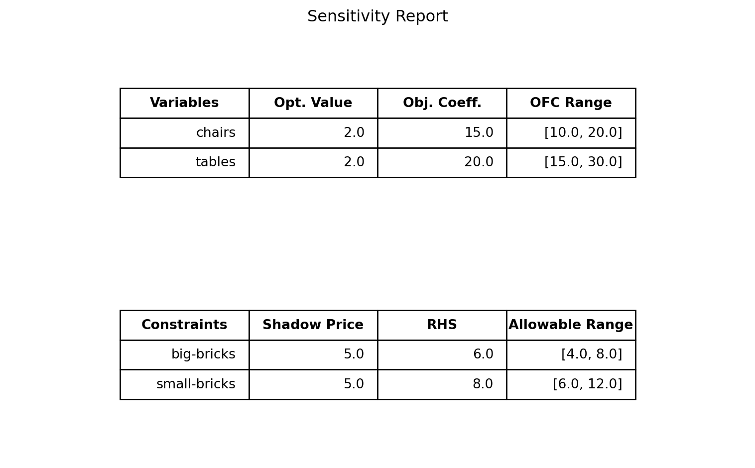
4.3 Beyond the basics
When building optimization models in gurobipy, you often need many decision variables and long sums in objectives or constraints. Instead of writing everything manually, Gurobi provides tools to do this compactly and clearly.
Two especially useful tools are:
addVars(): Create many variables at oncequicksum(): Efficiently create constraints in terms of decision variables
4.3.1 Defining many variables
If we define a Model() object with name problem, we can use the syntax x = problem.addVars(n) to tell Python to create n decision variables. You can use the i-th decision variable to define constraints and the objective function by indexing x at position i-1, i.e, by using x[i-1]. Recall that Python starts counting from zero when indexing data objects such as lists.
If you want you can also add a list of names for the decision variables using the name keyword argument. Make sure that the number of elements in the list matches the value of n.
Below we use addVars() to again define the Duplo example with n = 2.
from gurobipy import Model, GRB
# Initialize Gurobi model.
duplo = Model(name='Duplo problem')
# Declare the two decision variables using addVars()
x = duplo.addVars(2,name=["chairs","tables"])
# Specify the objective function in terms of x[0] and x[1]
duplo.setObjective(15*x[0] + 20*x[1], sense=GRB.MAXIMIZE)
# Add the resource constraints on bricks in terms of x[0] and x[1]
duplo.addConstr(x[0] + 2*x[1] <= 6, name='big-bricks')
duplo.addConstr(2*x[0] + 2*x[1] <= 8, name='small-bricks')
# Optimize the duplo
duplo.optimize()4.3.2 Defining constraints quickly
The function quicksum() is convenient to use if you you want to add the objective function c_1x_1 + x_2x_2 + \dots + c_nx_n or a constraint of the form a_1x_1 + a_2x_2 + \dots + a_nx_n \leq b. You have to import this function into Python just as we have to do with Model and GRB.
Let us again consider the Duplo example. If we define x = [x_1, x_2] and c = [c_1, c_2] = [2, 2], then we can create the objective function c_1x_1 + c_2x_2 by first creating the list [c_1x_1, c_2x_2], containing the individual terms of the objective function, and then summing up the elements in this list. The latter is precisely what quicksum() does: It takes as input a list and adds up the number in this list.
In the code below we do two things:
- Create the list
y = [c[0]*x[0], c[1]*x[1]]using the concept of list comprehension. - Use the
quicksum()function to add up the elements in the listyand set the resulting variableobjas our objective function.
from gurobipy import Model, GRB, quicksum
# Initialize Gurobi model.
duplo = Model(name='Duplo problem')
# Declare the two decision variables using addVars()
x = duplo.addVars(2,name=["chairs","tables"])
# Coefficients of objective function
c = [2,2]
# Define list [c[0]*x[0], c[1]*x[1]]
y = [c[j]*x[j] for j in range(2)]
# Sum up the terms in the list y
obj = quicksum(y)
# Define objective
duplo.setObjective(obj, sense=GRB.MAXIMIZE) The part [c[j]*x[j] for j in range(2)] is the compact list comprehension syntax for creating [c[0]*x[0], c[1]*x[1]]. Recall from Section 3.5 that j in range(0,2) means we iterate over the values j = 0 and j = 1 (the value 2 is not included).
This time we are only creating a list with two elements, but imagine then if you have 100 variables, then [c[j]*x[j] for j in range(100)] would be all you need to create an objective function of the form c_1x_1 + c_2x_2 + \dots + c_{100}x_{100} which consists of 100 terms!
We remark that you can also combine the above steps into a more compact code that carries out the last three lines in one line.
# Define objective
duplo.setObjective(quicksum(c[j]*x[j] for j in range(2)), sense=GRB.MAXIMIZE) In a similar fashion you can define the left hand side of a constraint a_1x_1 + a_2x_2 + \dots + a_nx_n \leq b quickly with quicksum(). Below we have given the Duplo example implemented with the use of quicksum() and addVars().
from gurobipy import Model, GRB
# Initialize Gurobi model.
duplo = Model(name='Duplo problem')
# Declare the two decision variables using addVars()
x = duplo.addVars(2,name=["chairs","tables"])
# Objective function coefficients
c = [2,2]
# Big brick coefficients
b = [1,2]
# Small brick coefficients
s = [2,2]
# Specify the objective function in terms of x[0] and x[1]
duplo.setObjective(quicksum(c[j]*x[j] for j in range(2)), sense=GRB.MAXIMIZE)
# Add the resource constraints on bricks in terms of x[0] and x[1]
duplo.addConstr(quicksum(b[j]*x[j] for j in range(2)) <= 6, name='big-bricks')
duplo.addConstr(quicksum(s[j]*x[j] for j in range(2)) <= 8, name='small-bricks')
# Optimize the duplo
duplo.optimize()
# Print optimal values of decision variables
for var in duplo.getVars():
print(var.VarName, "=", var.X)Gurobi Optimizer version 12.0.1 build v12.0.1rc0 (win64 - Windows 10.0 (19045.2))
CPU model: 12th Gen Intel(R) Core(TM) i7-1265U, instruction set [SSE2|AVX|AVX2]
Thread count: 10 physical cores, 12 logical processors, using up to 12 threads
Optimize a model with 2 rows, 2 columns and 4 nonzeros
Model fingerprint: 0x1b7dc040
Coefficient statistics:
Matrix range [1e+00, 2e+00]
Objective range [2e+00, 2e+00]
Bounds range [0e+00, 0e+00]
RHS range [6e+00, 8e+00]
Presolve time: 0.00s
Presolved: 2 rows, 2 columns, 4 nonzeros
Iteration Objective Primal Inf. Dual Inf. Time
0 4.0000000e+30 3.500000e+30 4.000000e+00 0s
2 8.0000000e+00 0.000000e+00 0.000000e+00 0s
Solved in 2 iterations and 0.00 seconds (0.00 work units)
Optimal objective 8.000000000e+00
chairs = 2.0
tables = 2.04.4 Integer variables
If you are not interested in finding fractional solutions, but want to enforce the decision variables to take integer values, you can do this with the vtype keyword argument.
Consider the following linear optimization problem (without integrality constraints).
\begin{array}{lrrrrrrl} \max & z = & 2x_{1} &+ &x_{2} & & & \\ \text{s.t. } & &x_1 &+ & x_2& \leq & 2.5 & \\ & &x_1, & & x_2 & \geq & 0 & \end{array},
# Initialize Gurobi model.
model_frac = Model(name='Fractional problem')

# Suppress Gurobi Optimizer output
model_frac.setParam('OutputFlag',0)

# Declare the two decision variables.
x1 = model_frac.addVar(name="x1")
x2 = model_frac.addVar(name="x2")

# Specify the objective function.
model_frac.setObjective(2*x1 + x2, sense=GRB.MAXIMIZE)

# Add the resource constraints on bricks.
model_frac.addConstr(x1 + x2 <= 2.5)

# Optimize the model
model_frac.optimize()

# Print optimal values of decision variables
for var in model_frac.getVars():
    print(var.VarName, "=", var.X)
x1 = 2.5
x2 = 0.0If we specify vtype=GRB.INTEGER in the addVar() method when creating the variables, Gurobi will find an optimal solution with all decision variables being integers.
# Initialize Gurobi model.
model_int = Model(name='Integer problem')

# Suppress Gurobi Optimizer output
model_int.setParam('OutputFlag',0)

# Declare the two decision variables.
x1 = model_int.addVar(name="x1",vtype=GRB.INTEGER)
x2 = model_int.addVar(name="x2",vtype=GRB.INTEGER)

# Specify the objective function.
model_int.setObjective(2*x1 + x2, sense=GRB.MAXIMIZE)

# Add the resource constraints on bricks.
model_int.addConstr(x1 + x2 <= 2.5)

# Optimize the model
model_int.optimize()

# Print optimal values of decision variables
for var in model_int.getVars():
    print(var.VarName, "=", var.X)
x1 = 2.0
x2 = -0.0Anoter common case is where the decision variables are supposed to be binary, meaning they can only take values in \{0,1\}. Setting variables to be binary can be done with vtype=GRB.BINARY.
# Initialize Gurobi model.
model_bin = Model(name='Binary problem')

# Suppress Gurobi Optimizer output
model_bin.setParam('OutputFlag',0)

# Declare the two decision variables.
x1 = model_bin.addVar(name="x1",vtype=GRB.BINARY)
x2 = model_bin.addVar(name="x2",vtype=GRB.BINARY)

# Specify the objective function.
model_bin.setObjective(2*x1 + x2, sense=GRB.MAXIMIZE)

# Add the resource constraints on bricks.
model_bin.addConstr(x1 + x2 <= 2.5)

# Optimize the model
model_bin.optimize()

# Print optimal values of decision variables
for var in model_bin.getVars():
    print(var.VarName, "=", var.X)
x1 = 1.0
x2 = 1.0